Multiple imputation for three-level and cross-classified data
January 3, 2019Multiple imputation (MI) of missing values in hierarchical data can be tricky when the data do not have a simple two-level structure. In such a case, understanding and accounting for the hierarchical structure of the data can be challenging, and tools to handle these types of data are relatively rare.
In this post, I show and explain how to conduct MI for three-level and cross-classified data in R.
Types of hierarchical data
Hierarchical data have a clustered structure in the sense that observations are clustered in higher-level units (e.g., observations in persons, persons in groups). Here, I consider two types of this: nested and cross-classified data.
Nested data
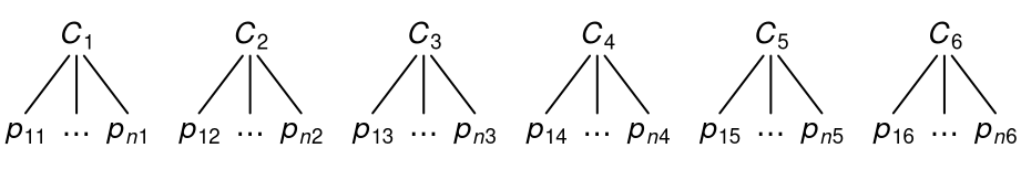
In nested data, every observation belongs to one and only one higher-level unit. Two-level data are a simple example for this type data, as shown below for six clusters with \(n\) observations.
More deeply nested structures are possible. For example, in three-level data, the clusters themselves are nested in even-higher-level units (e.g., students nested in classrooms nested in schools).
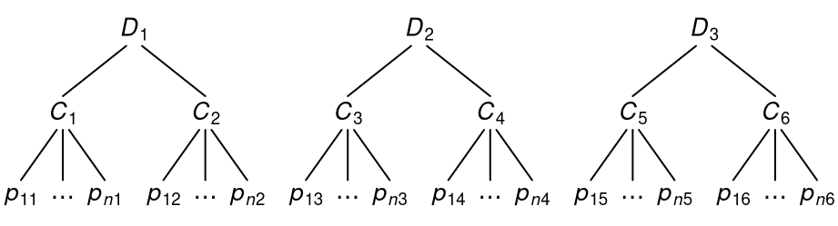
Here, observations \(p\) are nested within clusters \(C\), and clusters are nested within higher-level clusters \(D\).
Cross-classified data
In cross-classified data, every observation belongs directly to two or more clusters at once (e.g., experimental data with observations clustered within subjects and stimuli). However, the clusters are not themselves nested within one another but “crossed” as shown below.
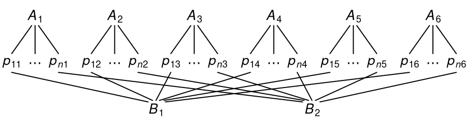
In contrast to nested data, there is no clear hierarchy of the two cluster variables. Differently put, although both \(A\) and \(B\) have observations clustered within them, neither of the two is itself nested within the other.
Why bother?
For the treatment of missing data, the hierarchical structure must be taken into account when using model-based methods such as MI (Enders, Mistler, & Keller, 2016; Lüdtke, Robitzsch, & Grund, 2017). This means that we need to acknowledge that, in hierarchical data, variables can vary both within and between clusters, and multiple variables can be related at each level of the structure.
Several articles have considered the case with two-level data (e.g., the two above). In the following, I show two examples for how to conduct MI for three-level and cross-classified data in R.
Three-level data
Suppose we have data from students (level 1) nested in classrooms (level 2) nested in schools (level 3) on four variables \(x\), \(y\), \(z\), and \(w\), where \(x\) and \(y\) are measured at level 1, \(z\) at level 2, and \(w\) at level 3. Consider the following model. For student \(i\), classroom \(j\), and school \(k\),
\[ y_{ijk} = \beta_0 + \beta_1 x_{ijk} + \beta_2 \bar{x}_{\bullet jk} + \beta_3 z_{jk} + \beta_4 \bar{x}_{\bullet \bullet k} + \beta_5 \bar{z}_{\bullet k} + \beta_6 w_k + u_{jk} + v_k + e_{ijk} \; , \]
where \(\bar{x}_{\bullet jk}\) and \(\bar{x}_{\bullet \bullet k}\) are the classroom and school mean of \(x\), \(\bar{z}_{\bullet k}\) is the school mean of \(z\), and \(u_{jk}\) and \(v_k\) are random intercepts at the classroom and school level, respectively. A graphical representation of the model is as follows.
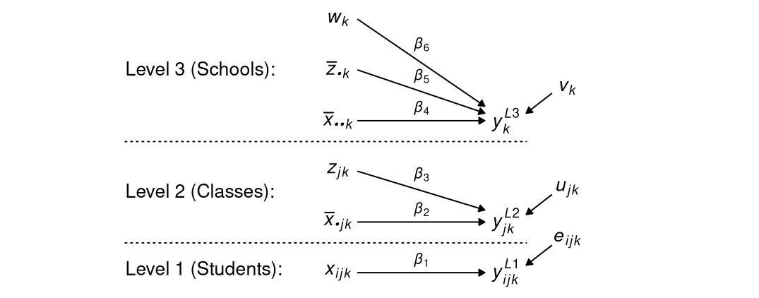
Notice how this model allows (a) for lower-level variables to have variance at the different levels, and (b) for the for the variables to be related to each other to different extents at each level. These features must be taken into account when conducting MI.
Example data
For this example, I simulated data with a three-level structure consisting of 50 schools (level 3), five classrooms per school (level 2), and 10 students per classroom (level 1, total \(n\) = 2500). The data can be downloaded here (CSV, Rdata).
| class | school | x | y | z | w |
|---|---|---|---|---|---|
| 1 | 1 | 0.318 | -0.261 | 0.456 | 1.33 |
| 1 | 1 | -0.251 | NA | 0.456 | 1.33 |
| 1 | 1 | -0.648 | NA | 0.456 | 1.33 |
| … | |||||
| 2 | 1 | -0.320 | NA | NA | 1.33 |
| 2 | 1 | 0.069 | 0.548 | NA | 1.33 |
| 2 | 1 | NA | NA | NA | 1.33 |
| … | |||||
| 250 | 50 | 1.339 | 1.451 | -0.630 | NA |
| 250 | 50 | 0.441 | 0.943 | -0.630 | NA |
| 250 | 50 | 0.775 | 0.568 | -0.630 | NA |
Every row corresponds to one student, and the classrooms and schools are numbered consecutively. All variables in the data set contain missing data.
Multiple imputation
To perform MI, I use the R packages mice and miceadds.
The mice package treats missing data by iterating through a sequence of imputation models, thus treating variable after variable in a step-by-step manner (for a general introduction to mice, see van Buuren & Groothuis-Oudshoorn, 2011).
The imputation models are set up by defining (a) a method for each variable, naming the type of model to be used, and (b) a predictor matrix, naming which predictors (columns) should be used for each variable (rows). Extracting the defaults provides a good starting point.
library(mice)
library(miceadds)

# predictor matrix and imputation method (defaults)
predMatrix <- make.predictorMatrix(data = dat)
impMethod <- make.method(data = dat)
By default, mice uses methods intended for non-hierarchical data.
For multilevel data, we need to ensure that the imputation model takes the multilevel structure into account such that the models will need to include variance components at higher levels and allow for different relations between variables at different levels.
Setting up imputation models
To this end, we use (a) the ml.lmer method from miceadds to impute the lower-level variables x, y, and z, and (b) the 2lonly.norm method from mice to impute w at the “top” of the hierarchy.
# method for lower-level variables (x, y, and z)
impMethod[c("x", "y", "z")] <- "ml.lmer"

# method for variables at top level (w)
impMethod["w"] <- "2lonly.norm"
The two methods require that the hierarchical structure of the imputation model is set up in different ways. To make this easier, we first remove the cluster indicators from the set of predictors altogether by setting their column values to zero.
# remove indicator variables from predictor matrix
predMatrix[, c("class", "school")] <- 0
For variables imputed with 2lonly.norm, the hierarchical structure is relatively simple and can be specified in the predictor matrix by setting the highest-level cluster indicator to -2.
Here, the “top” indicator is school.
# ... specify cluster indicator (2lonly.norm)
predMatrix["w", "school"] <- -2
For variables imputed with ml.lmer, the hierarchical structure can be more complicated and must be set with two additional arguments (i.e., outside the predictor matrix).
First, for all higher-level variables (e.g., z and w), we need to specify the level at which the variables are measured (all others are assumed to be measured at level 1).
# ... specify levels of higher-level variables
level <- character(ncol(dat))
names(level) <- colnames(dat)

level["w"] <- "school"
level["z"] <- "class"
Second, for each variable, we need to specify the cluster variables that define the hierarchical structure in the imputation model. By default, this uses a random intercept model with random effects at each of the specified levels.
# ... specify cluster indicators (as list)
cluster <- list()

cluster[["x"]] <- c("class", "school")
cluster[["y"]] <- c("class", "school")
cluster[["z"]] <- c("school")
Notice that we did not have to specify at which level the variables are meant to predict one another.
This is because both ml.lmer and 2lonly.norm will calculate and include any aggregates of lower-level variables at higher levels whenever possible, meaning that the relations between variables at different levels are automatically included in the imputation models.
Imputation
To start the imputation, we can now run mice as follows.
# run mice
imp <- mice(dat, method = impMethod, predictorMatrix = predMatrix, maxit = 20,
            m = 20, levels_id = cluster, variables_levels = level)
This generates 20 imputations for the missing data.
Example analysis
I use the R packages mitml and lme4 to analyze the imputed data.
First, I extract a list imputed data sets and calculate the cluster means that we need in order to fit the analysis model.
library(mitml)

# create list of imputed data sets
implist <- mids2mitml.list(imp)

# calculate group means
implist <- within(implist, {
  x.cls <- clusterMeans(x, class)
  x.sch <- clusterMeans(x, school)
})
The analysis model is then fitted with the lme4 package, and the results are pooled with mitml with the following lines of code.
library(lme4)

# fit model
fit <- with(implist,{
  lmer(y ~ 1 + x + x.cls + x.sch + z + w + (1|class) + (1|school))
})

# pool results
testEstimates(fit, var.comp = TRUE)
#
# Call:
#
# testEstimates(model = fit, var.comp = TRUE)
#
# Final parameter estimates and inferences obtained from 20 imputed data sets.
#
# Estimate Std.Error t.value df P(>|t|) RIV FMI
# (Intercept) -0.025 0.082 -0.306 3462.095 0.760 0.080 0.075
# x 0.190 0.019 10.186 113.399 0.000 0.693 0.419
# x.cls 0.460 0.058 7.968 220.257 0.000 0.416 0.300
# x.sch 0.352 0.149 2.359 3807.532 0.018 0.076 0.071
# z -0.135 0.028 -4.774 363.762 0.000 0.296 0.233
# w -0.071 0.083 -0.860 446.933 0.390 0.260 0.210
#
# Estimate
# Intercept~~Intercept|class 0.084
# Intercept~~Intercept|school 0.247
# Residual~~Residual 0.312
#
# Unadjusted hypothesis test as appropriate in larger samples.These results are very close to the parameters I used to generate the data. In the next example, we move on to clustered data with a cross-classified structure.
Cross-classified data
Suppose that we ran an experiment, in which subjects responded to items or stimuli, and obtained data for three variables \(y\), \(a\), and \(z\), where \(y\) is the outcome at level 1, \(a\) is a binary variable at the item level representing the experimental conditions, and \(b\) is a covariate at the person level. Our model of interest is as follows. For response \(i\) of subject \(j\) on item \(k\)
\[ y_{ijk} = \beta_0 + \beta_1 z_j + \beta_2 a_k + u_j + v_k + e_{ijk} \; , \]
where \(u_j\) and \(v_k\) denote random effects for subjects and items, respectively. The model can be illustrated like this.

You can see that this model is relatively simple because it does not contain aggregated variables.1 Nonetheless, it allows for (a) an effect of the experimental condition at the item level, (b) relations with the covariate at the person level, and (c) residual variance in the outcome at the level of items, subjects, and responses (i.e., in the interaction of items and subjects).
Notice how there is no “third” level in this model. Instead, the “top” level includes both subjects and items, which are not further nested in one another.
Example data
For this example, I simulated data with a cross-classified structure and a total of \(n\) = 5000 responses (level 1) from 100 subjects (level 2b) to 50 items (level 2a). The experimental condition (\(a\) = 1) comprised all even-numbered items; the control (\(a\) = 0) all the odd-numbered items. The data can be downloaded here (CSV, Rdata).
| item | subject | y | a | z |
|---|---|---|---|---|
| 1 | 1 | 0.263 | 0 | -1.18 |
| 2 | 1 | 2.029 | 1 | -1.18 |
| 3 | 1 | NA | 0 | -1.18 |
| … | ||||
| 48 | 100 | 0.285 | 1 | -1.32 |
| 49 | 100 | -1.781 | 0 | -1.32 |
| 50 | 100 | -0.202 | 1 | -1.32 |
Some of the responses (\(y\)) are sporadically missing. In addition, a number of subjects failed to provide data on the subject-level covariate (\(z\)).
Multiple imputation
The main strategy for MI remains the same as in the previous example. In order to accommodate the multilevel structure, we again need to ensure that the imputation model allows for the variables to have variance and relations with each other at different levels, with the exception that aggregated variables are not used here (see Footnote 1).
We again start with the default setup and adjust it the way we need to.
# create default predictor matrix and imputation methods
predMatrix <- make.predictorMatrix(data = dat)
impMethod <- make.method(data = dat)
Setting up imputation models
In this example, only y and z contain missing data.
For the lower-level variable y, we again use the ml.lmer method.
For z, we use 2lonly.norm because it is located at the “top” of the hierarchy (despite it not being there alone).2
# method for lower-level variables (y)
impMethod["y"] <- "ml.lmer"

# ... for variables at top level (z)
impMethod["z"] <- "2lonly.norm"
To set up these methods, we begin by removing the cluster indicators from the predictor matrix.
# remove indicator variables from set of predictors
predMatrix[, c("subject", "item")] <- 0
For variables imputed with 2lonly.norm, the hierarchical structure is then specified in the predictor matrix by setting its cluster indicator to -2.
The cluster indicator for z is subject.
# specify cluster indicator (2lonly.norm)
predMatrix["z", "subject"] <- -2
For variables imputed with ml.lmer, the setup again requires a few extra arguments.
Specifically, we need to specify (a) the level at which the higher-level variables (a and z) are measured and (b) the cluster variables that define the clustered structure in the imputation model of y.
# specify levels of higher-level variables
level <- character(ncol(dat))
names(level) <- colnames(dat)

level["a"] <- "item"
level["z"] <- "subject"

# specify cluster indicators (as list)
cluster <- list()

cluster[["y"]] <- c("subject", "item")
Recall that ml.lmer and 2lonly.norm automatically calculate and include any aggregated variables in every step of the imputation.
However, in this cross-classified design these aggregates turn out to be constant because every person responds to every item (see Footnote 1).
For this reason, the aggregates need to be removed from the imputation model.
For variables imputed with 2lonly.norm, we can do this by removing variables from the predictor matrix.
For z, we remove a from the set of predictors such that z is only predicted by the subject-level aggregate of y (but not a).
# remove effect of (average) a on z
predMatrix["z", "a"] <- 0
For variables imputed with ml.lmer, this is not done in the predictor matrix but with a global argument when running the imputation.3
Imputation
To start the imputation, we run mice as follows.
To turn off the automatic aggregation of variables used by ml.lmer, I also set the argument aggregate_automatically = FALSE.
# run mice
imp <- mice(dat, method = impMethod, predictorMatrix = predMatrix, maxit = 20,
            m = 20, levels_id = cluster, variables_levels = level,
            aggregate_automatically = FALSE)
Example analysis
The analysis of the data is done with lme4 and mitml as before.
First, we extract the imputed data sets as a list.
# create list of imputed data sets
implist <- mids2mitml.list(imp)
Then we fit the analysis model with lme4 and pool the results with mitml.
# fit model
fit <- with(implist,{
  lmer(y ~ 1 + a + z + (1|item) + (1|subject))
})

# pool results
testEstimates(fit, var.comp = TRUE)
#
# Call:
#
# testEstimates(model = fit, var.comp = TRUE)
#
# Final parameter estimates and inferences obtained from 20 imputed data sets.
#
# Estimate Std.Error t.value df P(>|t|) RIV FMI
# (Intercept) -0.161 0.106 -1.514 154490.706 0.130 0.011 0.011
# a 0.659 0.124 5.324 2581059.039 0.000 0.003 0.003
# z -0.248 0.072 -3.469 361.838 0.001 0.297 0.233
#
# Estimate
# Intercept~~Intercept|subject 0.341
# Intercept~~Intercept|item 0.186
# Residual~~Residual 0.462
#
# Unadjusted hypothesis test as appropriate in larger samples.The results are again close to the true values I used to generate the data.
Final remarks
In two examples, I showed how to conduct MI for three-level and cross-classified data in R.
In both cases, the hierarchical structure of the data and the relations that exist between variables at different levels of the structure have to be taken into account in the imputation model.
This ensures that the imputations are in line with the posited structure of the data, without which MI might lead to biased results.
We saw that this requires that we (a) choose appropriate imputation methods for hierarchical data (e.g., those in mice and miceadds) and (b) include aggregated versions of variables into the imputation model.
Notice that, although the two types of hierarchical data are very different, the ideas for treating missing data therein were similar. This is because, the random effects used to represent the hierarchical structure are additive in both cases. In fact, the same techniques can be used to treat missing data in any application where that is the case (e.g., nested data with four or more levels, more complex cross-classification, or a combination of the two).
The examples presented here used simulated continuous data. Similar methods are available for binary, ordinal, and (to some extent) polytomous data.
Further reading
- Enders, Mistler, and Keller (2016) and Lüdtke, Robitzsch, and Grund (2017) provide a general introduction to missing data and MI in hierarchical data with an emphasis on two-level data.
- Further examples for the imputation of three-level data with
miceandmiceaddscan be found in the documentation of themiceaddspackage. - The Blimp software (Keller & Enders, 2018) also supports MI for three-level data with some examples shown here.
References
- Enders, C. K., Mistler, S. A., & Keller, B. T. (2016). Multilevel multiple imputation: A review and evaluation of joint modeling and chained equations imputation. Psychological Methods, 21, 222–240. doi:10.1037/met0000063
- Keller, B. T., & Enders, C. K. (2018). Blimp Software Manual (Version 1.1).
- Lüdtke, O., Robitzsch, A., & Grund, S. (2017). Multiple imputation of missing data in multilevel designs: A comparison of different strategies. Psychological Methods, 22, 141–165. doi:10.1037/met0000096
- van Buuren, S., & Groothuis-Oudshoorn, K. (2011). MICE: Multivariate imputation by chained equations in R. Journal of Statistical Software, 45(3), 1–67. doi:10.18637/jss.v045.i03
In the present case, aggregating \(a\) and \(z\) is not useful, because all items are answered by all subjects, so that the aggregates of \(a\) at the person level and \(z\) at the item level are constant (e.g., every person responds to the same number of items in the experimental and the control condition). However, aggregated variables can still play a role in cross-classified data. For example, there can be other variables at level 1 (e.g., a covariate providing information about individual trials) or the experimental manipulation may be applied at level 1 (e.g., if it is applied randomly to items on a trial-by-trial basis). In such a case, the aggregated of these variables would not be constant and may need to be taken into account during MI.↩︎
If the item-level variable \(a\) also had missing data, we would treat it the same way (i.e., with
2lonly.norm) but specify a different cluster indicator in the predictor matrix (i.e.,item).# specify imputation method impMethod["a"] <- "2lonly.norm" # specify cluster indicator predMatrix["a", "item"] <- -2This is not needed here because
ahas no missing data.↩︎If there are other variables that need to be aggregated (e.g., other variables at level 1), then the aggregation needs to be done “by hand”, either by calculating the aggregated variables beforehand (if the variables are completely observed) or by using “passive imputation” (if they are incomplete).↩︎